
文档简介:


自然语言情感分析和文本匹配是日常生活中最常用的两类自然语言处理任务,本节主要介绍情感分析和文本匹配原理实现和典型模型,以及如何使用飞桨完成情感分析任务。
自然语言情感分析
人类自然语言具有高度的复杂性,相同的对话在不同的情景,不同的情感,不同的人演绎,表达的效果往往也会迥然不同。例如"你真的太瘦了",当你聊天的对象是一位身材苗条的人,这是一句赞美的话;当你聊天的对象是一位肥胖的人时,这就变成了一句嘲讽。感兴趣的读者可以看一段来自肥伦秀的视频片段,继续感受下人类语言情感的复杂性。
从视频中的内容可以看出,人类自然语言不只具有复杂性,同时也蕴含着丰富的情感色彩:表达人的情绪(如悲伤、快乐)、表达人的心情(如倦怠、忧郁)、表达人的喜好(如喜欢、讨厌)、表达人的个性特征和表达人的立场等等。利用机器自动分析这些情感倾向,不但有助于帮助企业了解消费者对其产品的感受,为产品改进提供依据;同时还有助于企业分析商业伙伴们的态度,以便更好地进行商业决策。
简单的说,我们可以将情感分析(sentiment classification)任务定义为一个分类问题,即指定一个文本输入,机器通过对文本进行分析、处理、归纳和推理后自动输出结论,如图1所示。
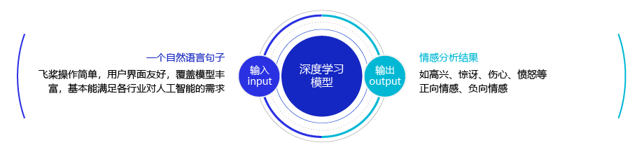
图1:情感分析任务
通常情况下,人们把情感分析任务看成一个三分类问题,如 图2 所示:

图2:情感分析任务
- 正向: 表示正面积极的情感,如高兴,幸福,惊喜,期待等。
- 负向: 表示负面消极的情感,如难过,伤心,愤怒,惊恐等。
- 其他: 其他类型的情感。
在情感分析任务中,研究人员除了分析句子的情感类型外,还细化到以句子中具体的“方面”为分析主体进行情感分析(aspect-level),如下:
这个薯片口味有点咸,太辣了,不过口感很脆。
关于薯片的口味方面是一个负向评价(咸,太辣),然而对于口感方面却是一个正向评价(很脆)。
我很喜欢夏威夷,就是这边的海鲜太贵了。
关于夏威夷是一个正向评价(喜欢),然而对于夏威夷的海鲜却是一个负向评价(价格太贵)。
使用深度神经网络完成情感分析任务
上一节课我们学习了通过把每个单词转换成向量的方式,可以完成单词语义计算任务。那么我们自然会联想到,是否可以把每个自然语言句子也转换成一个向量表示,并使用这个向量表示完成情感分析任务呢?
在日常工作中有一个非常简单粗暴的解决方式:就是先把一个句子中所有词的embedding进行加权平均,再用得到的平均embedding作为整个句子的向量表示。然而由于自然语言变幻莫测,我们在使用神经网络处理句子的时候,往往会遇到如下两类问题:
-
变长的句子: 自然语言句子往往是变长的,不同的句子长度可能差别很大。然而大部分神经网络接受的输入都是张量,长度是固定的,那么如何让神经网络处理变长数据成为了一大挑战。
-
组合的语义: 自然语言句子往往对结构非常敏感,有时稍微颠倒单词的顺序都可能改变这句话的意思,比如:
你等一下我做完作业就走。
我等一下你做完工作就走。
我不爱吃你做的饭。
你不爱吃我做的饭。
我瞅你咋地。
你瞅我咋地。
因此,我们需要找到一个可以考虑词和词之间顺序(关系)的神经网络,用于更好地实现自然语言句子建模。
处理变长数据
在使用神经网络处理变长数据时,需要先设置一个全局变量max_seq_len,再对语料中的句子进行处理,将不同的句子组成mini-batch,用于神经网络学习和处理。
1. 设置全局变量
设定一个全局变量max_seq_len,用来控制神经网络最大可以处理文本的长度。我们可以先观察语料中句子的分布,再设置合理的max_seq_len值,以最高的性价比完成句子分类任务(如情感分类)。
2. 对语料中的句子进行处理
我们通常采用 截断+填充 的方式,对语料中的句子进行处理,将不同长度的句子组成mini-batch,以便让句子转换成一个张量给神经网络进行计算,如 图 3 所示。
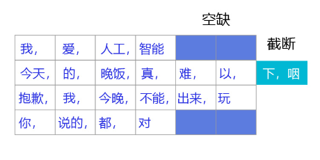
图3:变长数据处理
-
对于长度超过max_seq_len的句子,通常会把这个句子进行截断,以便可以输入到一个张量中。句子截断是有技巧的,有时截取句子的前一部分会比后一部分好,有时则恰好相反。当然也存在其他的截断方式,有兴趣的读者可以翻阅一下相关资料,这里不做赘述。
- 前向截断: “晚饭, 真, 难, 以, 下, 咽”
- 后向截断:“今天, 的, 晚饭, 真, 难, 以”
-
对于句子长度不足max_seq_len的句子,我们一般会使用一个特殊的词语对这个句子进行填充,这个过程称为Padding。假设给定一个句子“我,爱,人工,智能”,max_seq_len=6,那么可能得到两种填充方式:
- 前向填充: “[pad],[pad],我,爱,人工,智能”
- 后向填充:“我,爱,人工,智能,[pad],[pad]”
同样,不同的填充方式也对网络训练效果有一定影响。一般来说,后向填充是更常用的选择。
学习句子的语义
上一节课学习了如何学习每个单词的语义信息,从上面的举例中我们也会观察到,一个句子中词的顺序往往对这个句子的整体语义有重要的影响。因此,在刻画整个句子的语义信息过程中,不能撇开顺序信息。如果简单粗暴地把这个句子中所有词的向量做加和,会使得我们的模型无法区分句子的真实含义,例如:
我不爱吃你做的饭。
你不爱吃我做的饭。
一个有趣的想法,把一个自然语言句子看成一个序列,把自然语言的生成过程看成是一个序列生成的过程。例如对于句子“我,爱,人工,智能”,这句话的生成概率P(我,爱,人工,智能)\text{P}(\text{我,爱,人工,智能})P(我,爱,人工,智能)可以被表示为:
P(我,爱,人工,智能)=P(我∣)∗P(爱∣
,我)∗P(人工∣,我,爱)∗P(智能∣,我,爱,人工)
∗P(∣,我,爱,人工,智能)\text{P}(\text{我,爱,人工,智能})=\text{P}(我|\text{})
*\text{P}(爱|\text{,我})* \text{P}(人工|\text{,我,爱})* \text{P}(智能|\text{,我,
爱,人工})* \text{P}(\text{}|\text{,我,爱,人工,智能})P(我,爱,人工,智能)=P
(我∣)∗P(爱∣,我)∗P(人工∣,我,爱)∗P(智能∣,我,爱,人工)∗P(∣,我,爱,人工,智能)
其中\text{}和\text{
上面的公式把一个句子的生成过程建模成一个序列的决策过程,这就是香农在1950年左右提出的使用马尔可夫过程建模自然语言的思想。使用序列的视角看待和建模自然语言有一个明显的好处,那就是在对每个词建模的过程中,都有机会去学习这个词和之前生成的词之间的关系,并利用这种关系更好地处理自然语言。如 图4 所示,生成句子“我,爱,人工”后,“智能”在下一步生成的概率就变得很高了,因为“人工智能”经常同时出现。
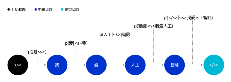
图4:自然语言生成过程示意图
通过考虑句子内部的序列关系,我们就可以清晰地区分“我不爱吃你做的菜”和“你不爱吃我做的菜”这两句话之间的联系与不同了。事实上,目前大多数成功的自然语言模型都建立在对句子的序列化建模上。下面让我们学习两个经典的序列化建模模型:循环神经网络(Recurrent Neural Network,RNN)和长短时记忆网络(Long Short-Term Memory,LSTM)。
循环神经网络RNN和长短时记忆网络LSTM
RNN和LSTM网络的设计思考
与读者熟悉的卷积神经网络(Convolutional Neural Networks, CNN)一样,各种形态的神经网络在设计之初,均有针对特定场景的奇思妙想。卷积神经网络的设计具备适合视觉任务“局部视野”特点,是因为视觉信息是局部有效的。例如在一张图片的1/4区域上有一只小猫,如果将图片3/4的内容遮挡,人类依然可以判断这是一只猫。
与此类似,RNN和LSTM的设计初衷是部分场景神经网络需要有“记忆”能力才能解决的任务。在自然语言处理任务中,往往一段文字中某个词的语义可能与前一段句子的语义相关,只有记住了上下文的神经网络才能很好的处理句子的语义关系。例如:
我一边吃着苹果,一边玩着苹果手机。
网络只有正确的记忆两个“苹果”的上下文“吃着”和“玩着…手机”,才能正确的识别两个苹果的语义,分别是水果和手机品牌。如果网络没有记忆功能,那么两个“苹果”只能归结到更高概率出现的语义上,得到一个相同的语义输出,这显然是不合理的。
如何设计神经网络的记忆功能呢?我们先了解下RNN网络是如何实现具备记忆功能的。RNN相当于将神经网络单元进行了横向连接,处理前一部分输入的RNN单元不仅有正常的模型输出,还会输出“记忆”传递到下一个RNN单元。而处于后一部分的RNN单元,不仅仅有来自于任务数据的输入,同时会接收从前一个RNN单元传递过来的记忆输入,这样就使得整个神经网络具备了“记忆”能力。
但是RNN网络只是初步实现了“记忆”功能,在此基础上科学家们又发明了一些RNN的变体,来加强网络的记忆能力。但RNN对“记忆”能力的设计是比较粗糙的,当网络处理的序列数据过长时,累积的内部信息就会越来越复杂,直到超过网络的承载能力,通俗的说“事无巨细的记录,总有一天大脑会崩溃”。为了解决这个问题,科学家巧妙的设计了一种记忆单元,称之为“长短时记忆网络(Long Short-Term Memory,LSTM)”。在每个处理单元内部,加入了输入门、输出门和遗忘门的设计,三者有明确的任务分工:
- 输入门:控制有多少输入信号会被融合;
- 遗忘门:控制有多少过去的记忆会被遗忘;
- 输出门:控制多少处理后的信息会被输出;
三者的作用与人类的记忆方式有异曲同工之处,即:
- 与当前任务无关的信息会直接过滤掉,如非常专注的开车时,人们几乎不注意沿途的风景;
- 过去记录的事情不一定都要永远记住,如令人伤心或者不重要的事,通常会很快被淡忘;
- 根据记忆和现实观察进行决策,如开车时会结合记忆中的路线和当前看到的路标,决策转弯或不做任何动作。
了解了这些关于网络设计的本质,下面进入实现方案的细节。
RNN网络结构
RNN是一个非常经典的面向序列的模型,可以对自然语言句子或是其它时序信号进行建模,网络结构如 图5 所示。
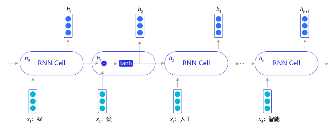
图5:RNN网络结构
不同于其他常见的神经网络结构,循环神经网络的输入是一个序列信息。假设给定任意一句话[x0,x1,...,xn][x_0, x_1, ..., x_n][x0,x1,...,xn],其中每个xix_ixi都代表了一个词,如“我,爱,人工,智能”。循环神经网络从左到右逐词阅读这个句子,并不断调用一个相同的RNN Cell来处理时序信息。每阅读一个单词,循环神经网络会先将本次输入的单词通过embedding lookup转换为一个向量表示。再把这个单词的向量表示和这个模型内部记忆的向量hhh融合起来,形成一个更新的记忆。最后将这个融合后的表示输出出来,作为它当前阅读到的所有内容的语义表示。当循环神经网络阅读过整个句子之后,我们就可以认为它的最后一个输出状态表示了整个句子的语义信息。
听上去很复杂,下面我们以一个简单地例子来说明,假设输入的句子为:
“我,爱,人工,智能”
循环神经网络开始从左到右阅读这个句子,在未经过任何阅读之前,循环神经网络中的记忆向量是空白的。其处理逻辑如下:
- 网络阅读单词“我”,并把单词“我”的向量表示和空白记忆相融合,输出一个向量h1h_1h1,用于表示“空白+我”的语义。
- 网络开始阅读单词“爱”,这时循环神经网络内部存在“空白+我”的记忆。循环神经网络会将“空白+我”和“爱”的向量表示相融合,并输出“空白+我+爱”的向量表示h2h_2h2,用于表示“我爱”这个短语的语义信息。
- 网络开始阅读单词“人工”,同样经过融合之后,输出“空白+我+爱+人工”的向量表示h3h_3h3,用于表示“空白+我+爱+人工”语义信息。
- 最终在网络阅读了“智能”单词后,便可以输出“我爱人工智能”这一句子的整体语义信息。
说明:
在实现当前输入xtx_txt和已有记忆ht−1h_{t-1}ht−1融合的时候,循环神经网络采用相加并通过一个激活函数tanh的方式实现:
ht=tanh(WXt+VHt−1+b)h_t = tanh(WX_{t}+VH_{t-1}+b)ht=tanh(WXt+VHt−1+b)
tanh函数是一个值域为(-1,1)的函数,其作用是长期维持内部记忆在一个固定的数值范围内,防止因多次迭代更新导致数值爆炸。同时tanh的导数是一个平滑的函数,会让神经网络的训练变得更加简单。
LSTM网络结构
上述方法听上去很有效(事实上在有些任务上效果还不错),但是存在一个明显的缺陷,就是当阅读很长的序列时,网络内部的信息会变得越来越复杂,甚至会超过网络的记忆能力,使得最终的输出信息变得混乱无用。长短时记忆网络(Long Short-Term Memory,LSTM)内部的复杂结构正是为处理这类问题而设计的,其网络结构如 图6 所示。
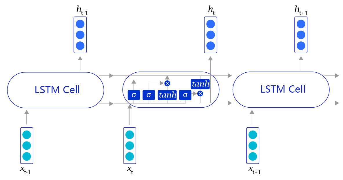
图6:LSTM网络结构
长短时记忆网络的结构和循环神经网络非常类似,都是通过不断调用同一个cell来逐次处理时序信息。每阅读一个新单词xtx_txt,就会输出一个新的输出信号hth_tht,用来表示当前阅读到所有内容的整体向量表示。不过二者又有一个明显区别,长短时记忆网络在不同cell之间传递的是两个记忆信息,而不像循环神经网络一样只有一个记忆信息,此外长短时记忆网络的内部结构也更加复杂,如 图7 所示。
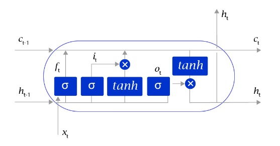
图7:LSTM网络内部结构示意图
区别于循环神经网络RNN,长短时记忆网络最大的特点是在更新内部记忆时,引入了遗忘机制。即容许网络忘记过去阅读过程中看到的一些无关紧要的信息,只保留有用的历史信息。通过这种方式延长了记忆长度。举个例子:
我觉得这家餐馆的菜品很不错,烤鸭非常正宗,包子也不错,酱牛肉很有嚼劲。但是服务员态度太恶劣了,我们在门口等了50分钟都没有能成功进去,好不容易进去了,桌子也半天没人打扫。整个环境非常吵闹,我的孩子都被吓哭了,我下次不会带朋友来。
当我们阅读上面这段话的时候,可能会记住一些关键词,如烤鸭好吃、牛肉有嚼劲、环境吵等,但也会忽略一些不重要的内容,如“我觉得”、“好不容易”等,长短时记忆网络正是受这个启发而设计的。
长短时记忆网络的Cell有三个输入:
- 这个网络新看到的输入信号,如下一个单词,记为xtx_{t}xt, 其中xtx_{t}xt是一个向量,ttt代表了当前时刻。
- 这个网络在上一步的输出信号,记为ht−1h_{t-1}ht−1,这是一个向量,维度同xtx_{t}xt相同。
- 这个网络在上一步的记忆信号,记为ct−1c_{t-1}ct−1,这是一个向量,维度同xtx_{t}xt相同。
得到这两个信号之后,长短时记忆网络没有立即去融合这两个向量,而是计算了权重。
- 输入门:it=sigmoid(WiXt+ViHt−1+bi)i_{t}=sigmoid(W_{i}X_{t}+V_{i}H_
- {t-1}+b_i)it=sigmoid(WiXt+ViHt−1+bi),控制有多少输入信号会被融合。
- 遗忘门:ft=sigmoid(WfXt+VfHt−1+bf)f_{t}=sigmoid(W_{f}X_{t}+V_
- {f}H_{t-1}+b_f)ft=sigmoid(WfXt+VfHt−1+bf),控制有多少过去的记忆会被遗忘。
- 输出门:ot=sigmoid(WoXt+VoHt−1+bo)o_{t}=sigmoid(W_{o}X_{t}+V
- _{o}H_{t-1}+b_o)ot=sigmoid(WoXt+VoHt−1+bo),控制最终输出多少融合了记忆的信息。
- 单元状态:gt=tanh(WgXt+VgHt−1+bg)g_{t}=tanh(W_{g}X_{t}+V_{g}H_
- {t-1}+b_g)gt=tanh(WgXt+VgHt−1+bg),输入信号和过去的输入信号做一个信息融合。
通过学习这些门的权重设置,长短时记忆网络可以根据当前的输入信号和记忆信息,有选择性地忽略或者强化当前的记忆或是输入信号,帮助网络更好地学习长句子的语义信息:
-
记忆信号:ct=ft⋅ct−1+it⋅gtc_{t} = f_{t} \cdot c_{t-1} + i_{t} \cdot g_{t}ct=ft⋅ct−1+it⋅gt
-
输出信号:ht=ot⋅tanh(ct)h_{t} = o_{t} \cdot tanh(c_{t})ht=ot⋅tanh(ct)
说明:
事实上,长短时记忆网络之所以能更好地对长文本进行建模,还存在另外一套更加严谨的计算和证明,有兴趣的读者可以翻阅一下引文中的参考资料进行详细研究。
# encoding=utf8 import re import random import tarfile import requests import numpy
as np import paddle from paddle.nn import Embedding import paddle.nn.functional as
F from paddle.nn import LSTM, Embedding, Dropout, Linear
def download(): # 通过python的requests类,下载存储在 # https://dataset.bj.bcebos.
com/imdb%2FaclImdb_v1.tar.gz的文件 corpus_url = "https://dataset.bj.bcebos.com/imdb%2FaclImdb
_v1.tar.gz" web_request = requests.get(corpus_url)
    corpus = web_request.content # 将下载的文件写在当前目录的aclImdb_v1.tar.gz文件内 with
open("./aclImdb_v1.tar.gz", "wb") as f:
        f.write(corpus)
    f.close()

download()
接下来,将数据集加载到程序中,并打印一小部分数据观察一下数据集的特点,代码如下:
def load_imdb(is_training): data_set = [] # aclImdb_v1.tar.gz解压后是一个目录
# 我们可以使用python的rarfile库进行解压 # 训练数据和测试数据已经经过切分,其中训练数据的地址为:
# ./aclImdb/train/pos/ 和 ./aclImdb/train/neg/,分别存储着正向情感的数据和负向情感的数据 #
我们把数据依次读取出来,并放到data_set里 # data_set中每个元素都是一个二元组,(句子,label),
其中label=0表示负向情感,label=1表示正向情感 for label in ["pos", "neg"]: with tarfil
e.open("./aclImdb_v1.tar.gz") as tarf:
            path_pattern = "aclImdb/train/" + label + "/.*\.txt$" if is_training \ else "
aclImdb/test/" + label + "/.*\.txt$" path_pattern = re.compile(path_pattern)
            tf = tarf.next() while tf != None: if bool(path_pattern.match(tf.name)):
                    sentence = tarf.extractfile(tf).read().decode()
                    sentence_label = 0 if label == 'neg' else 1 data_set.append((sentence, sentence_label))
                tf = tarf.next() return data_set

train_corpus = load_imdb(True)
test_corpus = load_imdb(False) for i in range(5):
    print("sentence %d, %s" % (i, train_corpus[i][0]))
    print("sentence %d, label %d" % (i, train_corpus[i][1]))
<>:13: DeprecationWarning: invalid escape sequence \.
<>:14: DeprecationWarning: invalid escape sequence \.
<>:13: DeprecationWarning: invalid escape sequence \.
<>:14: DeprecationWarning: invalid escape sequence \.
<>:13: DeprecationWarning: invalid escape sequence \.
<>:14: DeprecationWarning: invalid escape sequence \.
/tmp/ipykernel_714/751244768.py:13: DeprecationWarning: invalid escape sequence \.
  path_pattern = "aclImdb/train/" + label + "/.*\.txt$" if is_training \
/tmp/ipykernel_714/751244768.py:14: DeprecationWarning: invalid escape sequence \.
  else "aclImdb/test/" + label + "/.*\.txt$"
sentence 0, Zentropa has much in common with The Third Man, another noir-like film set
among the rubble of postwar Europe. Like TTM, there is much inventive camera work. There
is an innocent American who gets emotionally involved with a woman he doesn't really
understand, and whose naivety is all the more striking in contrast with the natives.

But I'd have to say that The Third Man has a more well-crafted storyline. Zentropa is
a bit disjointed in this respect. Perhaps this is intentional: it is presented as a
 dream/nightmare, and making it too coherent would spoil the effect.

This movie is unrelentingly grim--"noir" in more than one sense; one never sees the
 sun shine. Grim, but intriguing, and frightening.
sentence 0, label 1
sentence 1, Zentropa is the most original movie I've seen in years. If you like unique
thrillers that are influenced by film noir, then this is just the right cure for all
of those Hollywood summer blockbusters clogging the theaters these days. Von Trier's
follow-ups like Breaking the Waves have gotten more acclaim, but this is really his
best work. It is flashy without being distracting and offers the perfect combination
of suspense and dark humor. It's too bad he decided handheld cameras were the wave
of the future. It's hard to say who talked him away from the style he exhibits here,
but it's everyone's loss that he went into his heavily theoretical dogma direction instead.
sentence 1, label 1
sentence 2, Lars Von Trier is never backward in trying out new techniques. Some of
them are very original while others are best forgotten.

He depicts postwar Germany as a nightmarish train journey. With so many cities lying
in ruins, Leo Kessler a young American of German descent feels obliged to help in
their restoration. It is not a simple task as he quickly finds out.

His uncle finds him a job as a night conductor on the Zentropa Railway Line. His job
is to attend to the needs of the passengers. When the shoes are polished a chalk mark
is made on the soles. A terrible argument ensues when a passenger's shoes are not chalked
despite the fact they have been polished. There are many allusions to the German
 fanaticism of adherence to such stupid details.

The railway journey is like an allegory representing man's procession through
life with all its trials and tribulations. In one sequence Leo dashes through the back
carriages to discover them filled with half-starved bodies appearing to have just
escaped from Auschwitz . These images, horrible as they are, are fleeting as in a dream,
each with its own terrible impact yet unconnected.

At a station called Urmitz Leo jumps from the train with a parceled bomb. In view of
many by-standers he connects the bomb to the underside of a carriage. He returns to
his cabin and makes a connection to a time clock. Later he jumps from the train
(at high speed) and lies in the cool grass on a river bank. Looking at the stars
above he decides that his job is to build and not destroy. Subsequently as he sees
the train approaching a giant bridge he runs at breakneck speed to board the train
and stop the clock. If you care to analyse the situation it is a completely impossible
 task. Quite ridiculous in fact. It could only happen in a dream.

It's strange how one remembers little details such as a row of cups hanging on
 hooks and rattling away with the swaying of the train.

Despite the fact that this film is widely acclaimed, I prefer Lars Von Trier'
s later films (Breaking the Waves and The Idiots). The bomb scene described
above really put me off. Perhaps I'm a realist.
sentence 2, label 1
sentence 3, *Contains spoilers due to me having to describe some film techniques,
so read at your own risk!*

I loved this film. The use of tinting in some of the scenes makes it seem like an
old photograph come to life. I also enjoyed the projection of people on a back
screen. For instance, in one scene, Leopold calls his wife and she is projected
behind him rather than in a typical split screen. Her face is huge in the back
 and Leo's is in the foreground.

One of the best uses of this is when the young boys kill the Ravensteins on the train,
a scene shot in an almost political poster style, with facial close ups. It reminded me
of Battleship Potemkin, that intense constant style coupled with the spray of red to
convey tons of horror without much gore. Same with the scene when Katharina finds her
father dead in the bathtub...you can only see the red water on the side. It is one of
the things I love about Von Trier, his understatement of horror, which ends up making
 it all the more creepy.

The use of text in the film was unique, like when Leo's character is pushed by the word,
 "Werewolf." I have never seen anything like that in a film.

The use of black comedy in this film was well done. Ernst-Hugo Järegård is great as Leo
's uncle. It brings up the snickers I got from his role in the Kingdom (Riget.) This humor
makes the plotline of absurd anal retentiveness of train conductors against the terrible
backdrop of WW2 and all the chaos, easier to take. It reminds me of Riget in the way
the hospital administrator is trying to maintain a normalcy at the end of part one when
everything is going crazy. It shows that some people are truly oblivious to the awful
things happening around them. Yet some people, like Leo, are tuned in, but do nothing
 positive about it.

The voice over, done expertly well by Max von Sydow, is amusing too. It draws you into
 the story and makes you jump into Leo's head, which at times is a scary place to be.

The movie brings up the point that one is a coward if they don't choose a side. I see
the same idea used in Dancer in the Dark, where Bjork's character doesn't speak up
for herself and ends up being her own destruction. Actually, at one time, Von Trier
seemed anti-woman to me, by making Breaking the Waves and Dancer, but now I know his
male characters don't fare well either! I found myself at the same place during the
end of Dancer, when you seriously want the main character to rethink their actions,
but of course, they never do!
sentence 3, label 1
sentence 4, That was the first thing that sprang to mind as I watched the closing
credits to Europa make there was across the screen, never in my entire life have
I seen a film of such technical genius, the visuals of Europa are so impressive
that any film I watch in it's wake will only pale in comparison, forget your Michael
Bay, Ridley Scott slick Hollywood cinematography, Europa has more ethereal beauty
than anything those two could conjure up in a million years. Now I'd be the first
to hail Lars von Trier a genius just off the back of his films Breaking the Waves
and Dancer in the Dark, but this is stupid, the fact that Europa has gone un-noticed
by film experts for so long is a crime against cinema, whilst overrated rubbish like
Crouching Tiger, Hidden Dragon and Life is Beautiful clean up at the academy awards
(but what do the know) Europa has been hidden away, absent form video stores and
(until recently) any British TV channels.

The visuals in Europa are not MTV gloss; it's not a case of style over substance,
its more a case of substance dictating style. Much like his first film The Element
of Crime, von Trier uses the perspective of the main character to draw us into his
world, and much like Element, the film begins with the main character (or in the case
of Europa, we the audience) being hypnotized. As we move down the tracks, the voice
of the Narrator (Max von Sydow) counts us down into a deep sleep, until we awake in
Europa. This allows von Trier and his three cinematographers to pay with the
conventions of time and imagery, there are many scenes in Europa when a character
in the background, who is in black and white, will interact with a person in the
foreground who will be colour, von Trier is trying to show us how much precedence
the coloured item or person has over the plot, for instance, it's no surprise that
the first shot of Leopold Kessler (Jean-marc Barr) is in colour, since he is the
only character who's actions have superiority over the film.

The performances are good, they may not be on par with performances in later von
Trier films, but that's just because the images are sometimes so distracting that
you don't really pick up on them the first time round. But I would like to point
out the fantastic performance of Jean-Marc Barr in the lead role, whose blind idealism
is slowly warn down by the two opposing sides, until he erupts in the films final act.
Again, muck like The Element of Crime, the film ends with our hero unable to wake up
from his nightmare state, left in this terrible place, with only the continuing narration
of von Sydow to seal his fate. Europa is a tremendous film, and I cant help thinking what
a shame that von Trier has abandoned this way of filming, since he was clearly one of
the most talented visual directors working at that time, Europa, much like the rest of
his cinematic cannon is filled with a wealth of iconic scenes. His dedication to compos
ition and mise-en-scene is unrivalled, not to mention his use of sound and production
design. But since his no-frills melodramas turned out to be Breaking the Waves and Dancer
 in the Dark then who can argue, but it does seems like a waste of an imaginative talent. 10/10
sentence 4, label 1
一般来说,在自然语言处理中,需要先对语料进行切词,这里我们可以使用空格把每个句子切成若干词的序列,代码如下:
def data_preprocess(corpus): data_set = [] for sentence, sentence_label in corpus:
# 这里有一个小trick是把所有的句子转换为小写,从而减小词表的大小 # 一般来说这样的做法有助于效果提升
sentence = sentence.strip().lower()
        sentence = sentence.split(" ")

        data_set.append((sentence, sentence_label)) return data_set

train_corpus = data_preprocess(train_corpus)
test_corpus = data_preprocess(test_corpus)
print(train_corpus[:5])
print(test_corpus[:5]
在代码中我们使用了一个特殊的单词"[oov]"(out-of-vocabulary),用于表示词表中没有覆盖到的词。之所以使用"[oov]"这个符号,是为了处理某一些词,在测试数据中有,但训练数据没有的现象。
# 构造词典,统计每个词的频率,并根据频率将每个词转换为一个整数id def build_dict(corpus):
 word_freq_dict = dict() for sentence, _ in corpus: for word in sentence: if word not in word_freq_dict
                word_freq_dict[word] = 0 word_freq_dict[word] += 1 word_freq_dict = sorted(word_fre
q_dict.items(), key = lambda x:x[1], reverse = True)

    word2id_dict = dict()
    word2id_freq = dict() # 一般来说,我们把oov和pad放在词典前面,给他们一个比较小的id,这样比较方
便记忆,并且易于后续扩展词表 word2id_dict['[oov]'] = 0 word2id_freq[0] = 1e10 word2id_dict['[pad]'
] = 1 word2id_freq[1] = 1e10 for word, freq in word_freq_dict:
        word2id_dict[word] = len(word2id_dict)
        word2id_freq[word2id_dict[word]] = freq return word2id_freq, word2id_dict

word2id_freq, word2id_dict = build_dict(train_corpus)
vocab_size = len(word2id_freq)
print("there are totoally %d different words in the corpus" % vocab_size) for _, (word, word_id)
 in zip(range(10), word2id_dict.items()):
    print("word %s, its id %d, its word freq %d" % (word, word_id, word2id_freq[word_id]))
there are totoally 252173 different words in the corpus
word [oov], its id 0, its word freq 10000000000
word [pad], its id 1, its word freq 10000000000
word the, its id 2, its word freq 322174
word a, its id 3, its word freq 159949
word and, its id 4, its word freq 158556
word of, its id 5, its word freq 144459
word to, its id 6, its word freq 133965
word is, its id 7, its word freq 104170
word in, its id 8, its word freq 90521
word i, its id 9, its word freq 70477
在完成word2id词典假设之后,我们还需要进一步处理原始语料,把语料中的所有句子都处理成ID序列,代码如下:
# 把语料转换为id序列 def convert_corpus_to_id(corpus, word2id_dict): data_set = []
for sentence, sentence_label in corpus: # 将句子中的词逐个替换成id,如果句子中的词不在词表内,
则替换成oov # 这里需要注意,一般来说我们可能需要查看一下test-set中,句子oov的比例,
# 如果存在过多oov的情况,那就说明我们的训练数据不足或者切分存在巨大偏差,需要调整 sentence
= [word2id_dict[word] if word in word2id_dict \ else word2id_dict['[oov]'] for word in sentence]
        data_set.append((sentence, sentence_label)) return data_set

train_corpus = convert_corpus_to_id(train_corpus, word2id_dict)
test_corpus = convert_corpus_to_id(test_corpus, word2id_dict)
print("%d tokens in the corpus" % len(train_corpus))
print(train_corpus[:5])
print(test_corpus[:5])
接下来,我们就可以开始把原始语料中的每个句子通过截断和填充,转换成一个固定长度的句子,并将所有数据整理成mini-batch,用于训练模型,代码如下:
# 编写一个迭代器,每次调用这个迭代器都会返回一个新的batch,用于训练或者预测 def build_batch(word
2id_dict, corpus, batch_size, epoch_num, max_seq_len, shuffle = True, drop_last = True):
# 模型将会接受的两个输入: # 1. 一个形状为[batch_size, max_seq_len]的张量,sentence_batch,
代表了一个mini-batch的句子。 # 2. 一个形状为[batch_size, 1]的张量,sentence_label_batch,
每个元素都是非0即1,代表了每个句子的情感类别(正向或者负向) sentence_batch = []
    sentence_label_batch = [] for _ in range(epoch_num): #每个epoch前都shuffle一下数据,
有助于提高模型训练的效果 #但是对于预测任务,不要做数据shuffle if shuffle:
            random.shuffle(corpus) for sentence, sentence_label in corpus:
            sentence_sample = sentence[:min(max_seq_len, len(sentence))] if len(sentence_sample)
< max_seq_len: for _ in range(max_seq_len - len(sentence_sample)):
                    sentence_sample.append(word2id_dict['[pad]'])


            sentence_sample = [[word_id] for word_id in sentence_sample]

            sentence_batch.append(sentence_sample)
            sentence_label_batch.append([sentence_label]) if len(sentence_batch) == batch_size:
yield np.array(sentence_batch).astype("int64"), np.array(sentence_label_batch).astype("int64")
                sentence_batch = []
                sentence_label_batch = [] if not drop_last and len(sentence_batch) >
0: yield np.array(sentence_batch).astype("int64"), np.array(sentence_label_batch).
astype("int64") for batch_id, batch in enumerate(build_batch(word2id_dict, train
_corpus, batch_size=3, epoch_num=3, max_seq_len=30)):
    print(batch) break
(array([[[  3589],
        [   161],
        [     7],
        [     3],
        [    56],
        [   139],
        [    18],
        [     6],
        [   493],
        [    12],
        [   141],
        [    61],
        [  1633],
        [     6],
        [   123],
        [    37],
        [  3490],
        [    75],
        [     4],
        [  2627],
        [    86],
        [    73],
        [    87],
        [  1985],
        [     9],
        [   372],
        [    10],
        [   155],
        [    18],
        [    12]],

       [[  2860],
        [ 18561],
        [     3],
        [  2145],
        [    19],
        [     2],
        [ 31184],
        [    16],
        [     3],
        [  9103],
        [  6089],
        [     4],
        [   569],
        [  7778],
        [    42],
        [  8134],
        [ 33621],
        [   289],
        [     5],
        [ 29830],
        [    34],
        [     2],
        [  2672],
        [155021],
        [   339],
        [    31],
        [   569],
        [  9776],
        [ 64528],
        [     8]],

       [[     9],
        [    81],
        [   200],
        [    10],
        [   691],
        [    83],
        [  1091],
        [     8],
        [166276],
        [     4],
        [    26],
        [    71],
        [  3709],
        [   227],
        [    96],
        [    17],
        [    83],
        [   435],
        [  1303],
        [    46],
        [    10],
        [     7],
        [    32],
        [  1738],
        [     6],
        [ 32973],
        [166277],
        [    96],
        [    44],
        [    32]]]), array([[1],
       [1],
       [1]]))
# 定义一个用于情感分类的网络实例,SentimentClassifier class SentimentClassifier(paddle.nn.Layer):
def __init__(self, hidden_size, vocab_size, embedding_size, class_num=2, num_steps=128, num_l
ayers=1, init_scale=0.1, dropout_rate=None): # 参数含义如下: # 1.hidden_size,表示embedding-size,
hidden和cell向量的维度 # 2.vocab_size,模型可以考虑的词表大小 # 3.embedding_size,表示词向量的维度
# 4.class_num,情感类型个数,可以是2分类,也可以是多分类 # 5.num_steps,表示这个情感分析模型最大
可以考虑的句子长度 # 6.num_layers,表示网络的层数 # 7.dropout_rate,表示使用dropout过程中失活的神
经元比例 # 8.init_scale,表示网络内部的参数的初始化范围,长短时记忆网络内部用了很多Tanh,Sigmoid等
激活函数,\ # 这些函数对数值精度非常敏感,因此我们一般只使用比较小的初始化范围,以保证效果 super
(SentimentClassifier, self).__init__()
        self.hidden_size = hidden_size
        self.vocab_size = vocab_size
        self.embedding_size = embedding_size
        self.class_num = class_num
        self.num_steps = num_steps
        self.num_layers = num_layers
        self.dropout_rate = dropout_rate
        self.init_scale = init_scale # 声明一个LSTM模型,用来把每个句子抽象成向量 self.simple_l
stm_rnn = paddle.nn.LSTM(input_size=hidden_size, hidden_size=hidden_size, num_layers=num_layers)
# 声明一个embedding层,用来把句子中的每个词转换为向量 self.embedding = paddle.nn.Embedding(num_
embeddings=vocab_size, embedding_dim=embedding_size, sparse=False,
                                    weight_attr=paddle.ParamAttr(initializer=paddle.nn.initiali
zer.Uniform(low=-init_scale, high=init_scale))) # 声明使用上述语义向量映射到具体情感类别时所需
要使用的线性层 self.cls_fc = paddle.nn.Linear(in_features=self.hidden_size, out_features=self.class_num,
                             weight_attr=None, bias_attr=None) # 一般在获取单词的embedding后,
会使用dropout层,防止过拟合,提升模型泛化能力 self.dropout_layer = paddle.nn.Dropout(p=self.dr
opout_rate, mode='upscale_in_train') # forwad函数即为模型前向计算的函数,它有两个输入,分别为:
# input为输入的训练文本,其shape为[batch_size, max_seq_len] # label训练文本对应的情感标签,
其shape维[batch_size, 1] def forward(self, inputs): # 获取输入数据的batch_size batch_size =
inputs.shape[0] # 本实验默认使用1层的LSTM,首先我们需要定义LSTM的初始hidden和cell,这里我们
使用0来初始化这个序列的记忆 init_hidden_data = np.zeros(
            (self.num_layers, batch_size, self.hidden_size), dtype='float32')
        init_cell_data = np.zeros(
            (self.num_layers, batch_size, self.hidden_size), dtype='float32') # 将这些初始记
忆转换为飞桨可计算的向量,并且设置stop_gradient=True,避免这些向量被更新,从而影响训练效果
init_hidden = paddle.to_tensor(init_hidden_data)
        init_hidden.stop_gradient = True init_cell = paddle.to_tensor(init_cell_data)
        init_cell.stop_gradient = True # 对应以上第2步,将输入的句子的mini-batch转换为词向量
表示,转换后输入数据shape为[batch_size, max_seq_len, embedding_size] x_emb = self.embedding(inputs)
        x_emb = paddle.reshape(x_emb, shape=[-1, self.num_steps, self.embedding_size])
 # 在获取的词向量后添加dropout层 if self.dropout_rate is not None and self.dropout_rate > 0.0:
            x_emb = self.dropout_layer(x_emb) # 对应以上第3步,使用LSTM网络,把每个句子转换为语义向量
# 返回的last_hidden即为最后一个时间步的输出,其shape为[self.num_layers, batch_size, hidden_size]
rnn_out, (last_hidden, last_cell) = self.simple_lstm_rnn(x_emb, (init_hidden, init_cell))
# 提取最后一层隐状态作为文本的语义向量,其shape为[batch_size, hidden_size] last_hidden =
paddle.reshape(last_hidden[-1], shape=[-1, self.hidden_size]) # 对应以上第4步,将每个句子
的向量表示映射到具体的情感类别上, logits的维度为[batch_size, 2]
logits = self.cls_fc(last_hidden) return logits
paddle.seed(0)
random.seed(0)
np.random.seed(0) # 定义训练参数 epoch_num = 5 batch_size = 128 learning_rate = 0.0001
dropout_rate = 0.2 num_layers = 1 hidden_size = 256 embedding_size = 256 max_seq_len
= 128 vocab_size = len(word2id_freq) # 实例化模型 sentiment_classifier = SentimentClas
sifier(hidden_size, vocab_size, embedding_size, num_steps=max_seq_len, num_layers=num_
layers, dropout_rate=dropout_rate) # 指定优化策略,更新模型参数 optimizer = paddle.opti
mizer.Adam(learning_rate=learning_rate, beta1=0.9, beta2=0.999, parameters= sentiment_c
lassifier.parameters()) # 定义训练函数 # 记录训练过程中的损失变化情况,
可用于后续画图查看训练情况 losses = []
steps = [] def train(model): # 开启模型训练模式 model.train() # 建立训练数据生成器,
每次迭代生成一个batch,每个batch包含训练文本和文本对应的情感标签 train_loader = build_
batch(word2id_dict, train_corpus, batch_size, epoch_num, max_seq_len) for step, (
sentences, labels) in enumerate(train_loader): # 获取数据,并将张量转换为Tensor类型
sentences = paddle.to_tensor(sentences)
        labels = paddle.to_tensor(labels) # 前向计算,将数据feed进模型,
并得到预测的情感标签和损失 logits = model(sentences) # 计算损失 loss = F.cross_
entropy(input=logits, label=labels, soft_label=False)
        loss = paddle.mean(loss) # 后向传播 loss.backward() # 更新参数 optimizer.step()
# 清除梯度 optimizer.clear_grad() if step % 100 == 0: # 记录当前步骤的loss变化情况
 losses.append(loss.numpy()[0])
            steps.append(step) # 打印当前loss数值 print("step %d, loss %.3f" %
(step, loss.numpy()[0])) #训练模型 train(sentiment_classifier) # 保存模型,包含两部分:
模型参数和优化器参数 model_name = "sentiment_classifier" # 保存训练好的模型参数 paddle
.save(sentiment_classifier.state_dict(), "{}.pdparams".format(model_name)) # 保存优化器参数,
方便后续模型继续训练 paddle.save(optimizer.state_dict(), "{}.pdopt".format(model_name))
W0510 11:45:39.448099 714 gpu_context.cc:244] Please NOTE: device: 0, GPU Compute Capability:
7.0, Driver API Version: 10.1, Runtime API Version: 10.1
W0510 11:45:39.453817   714 gpu_context.cc:272] device: 0, cuDNN Version: 7.6.
step 0, loss 0.693
def evaluate(model): # 开启模型测试模式,在该模式下,网络不会进行梯度更新 model.eval()
# 定义以上几个统计指标 tp, tn, fp, fn = 0, 0, 0, 0 # 构造测试数据生成器 test_loader = build
_batch(word2id_dict, test_corpus, batch_size, 1, max_seq_len) for sentences, labels in tes
t_loader: # 将张量转换为Tensor类型 sentences = paddle.to_tensor(sentences)
        labels = paddle.to_tensor(labels) # 获取模型对当前batch的输出结果 logits = model
(sentences) # 使用softmax进行归一化 probs = F.softmax(logits) # 把输出结果转换为numpy array数组,
比较预测结果和对应label之间的关系,并更新tp,tn,fp和fn probs = probs.numpy() for i
in range(len(probs)): # 当样本是的真实标签是正例 if labels[i][0] == 1: # 模型预测是正例
f probs[i][1] > probs[i][0]:
                    tp += 1 # 模型预测是负例 else:
                    fn += 1 # 当样本的真实标签是负例 else: # 模型预测是正例 if probs[i][1] > probs[i][0]:
                    fp += 1 # 模型预测是负例 else:
                    tn += 1 # 整体准确率 accuracy = (tp + tn) / (tp + tn + fp + fn) #
输出最终评估的模型效果 print("TP: {}\nFP: {}\nTN: {}\nFN: {}\n".format(tp, fp, tn, fn))
    print("Accuracy: %.4f" % accuracy) # 加载训练好的模型进行预测,重新实例化一个模型,
然后将训练好的模型参数加载到新模型里面 saved_state = paddle.load("./sentiment_classifier.pdparams")
sentiment_classifier = SentimentClassifier(hidden_size, vocab_size, embedding_size,
num_steps=max_seq_len, num_layers=num_layers, dropout_rate=dropout_rate)
sentiment_classifier.load_dict(saved_state) # 评估模型 evaluate(sentiment_classifier)
文本匹配
借助相同的思路,我们可以很轻易的解决文本相似度计算问题,假设给定两个句子:
句子1:我不爱吃烤冷面,但是我爱吃冷面
句子2:我爱吃菠萝,但是不爱吃地瓜
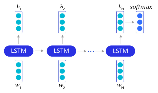
同样使用LSTM网络,把每个句子抽象成一个向量表示,通过计算这两个向量之间的相似度,就可以快速完成文本相似度计算任务。在实际场景里,我们也通常使用LSTM网络的最后一步hidden结果,将一个句子抽象成一个向量,然后通过向量点积,或者cosine相似度的方式,去衡量两个句子的相似度。
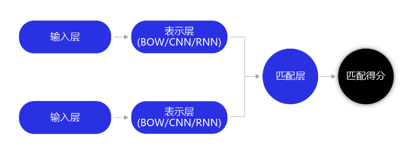
图9:文本相似度计算
一般情况下,在训练阶段有point-wise和pair-wise两个常见的训练模式(针对搜索引擎任务,还有一类list-wise的方法,这里不做探讨)。
-
point-wise训练模式: 在point-wise训练过程中,我们把不同的句子对儿分为两类(或者更多类别):相似、不相似。通过这种方式把句子相似度计算任务转化为了一个分类问题,通过常见的二分类函数(如sigmoid)即可完成分类任务。在最终预测阶段,使用sigmoid函数的输出,作为两个不同句子的相似度值。
-
pair-wise训练模式: pair-wise训练模式相对更复杂一些,假定给定3个句子,A,B和C。已知A和B相似,但是A和C不相似,那么原则上,A和B的相似度值应该高于A和C的相似度值。因此我们可以构造一个新的训练算法:对于一个相同的相似度计算模型mmm,假定m(A,B)m(A,B)m(A,B)是mmm输出的AAA和BBB的相似度值,m(A,C)是m(A,C)是m(A,C)是m输出的输出的输出的A和和和C$的相似度值,那么hinge-loss:
L=λ−(m(A,B)−m(A,C))L = \lambda - (m(A,B)-m(A,C))L=λ−(m(A,B)−m(A,C)) if m(A,B)−m(A,C)<λm(A,B)-m(A,C) < \lambdam(A,B)−m(A,C)<λ else 000
这个损失函数要求对于每个正样本m(A,B)m(A,B)m(A,B)的相似度值至少高于负样本m(A,C)m(A,C)m(A,C)一个阈值λ\lambdaλ。
hinge-loss的好处是没有强迫进行单个样本的分类,而是通过考虑样本和样本直接的大小关系来学习相似和不相似关系。相比较而言,pair-wise训练比point-wise任务效果更加鲁棒一些,更适合如搜索,排序,推荐等场景的相似度计算任务。
有兴趣的读者可以参考情感分析的模型实现,自行实现一个point-wise或pair-wise的文本相似度模型,相关数据集可参考文本匹配数据集。